Thompson Sampling vs. A/B testing

In this simulation, we'll dive into Thompson Sampling: the MAB algorithm behind how Coframe optimizes webpage copy and UI. We'll compare it to traditional A/B testing, highlighting how Thompson Sampling not only achieves higher cumulative rewards but also can test multiple variants (*arms*) simultaneously. By dynamically balancing exploration and exploitation, Thompson Sampling determines the best arm while reducing allocation to suboptimal variants.

First, some imports....

import numpy as np
import matplotlib.pyplot as plt
import pandas as pd
from scipy.stats import beta

For the sake of this demo, we'll assume that we have four possible variants, or arms, each with a different conversion rate. These will be unknown to the algorithm, but will be used to determine the rewards when each arm is tested. We'll also assume that we have the budget for 100k 'trials'. Think of a trial as showing one variant to a particular user, and the reward as a binary variable representing if a user was converted: 1 if they were, and 0 if they weren't.

# True conversion rates (unknown to the algorithm)
conversion_rates = [0.06, 0.09, 0.04, 0.03]
num_versions = len(conversion_rates)
num_trials = 100000

With both our A/B testing and Thompson Sampling algorithm, we'll use total conversions as our key metric:

A conversion could represent anything from a click to a sign-up to a purchase. We'll track and compare the conversion rates of Thompson Sampling and static A/B testing methods. In each case, our reward over time is the number of conversions across all trials so far.

A/B test

We'll start by defining a function to simulate an A/B test. Remember that when conducting an A/B test, we can only compare two versions at a time; we'll use the first two (note these are the two best variants of the 4!).

In each trial, we'll randomly select a variant to show to the user. We'll model the reward as a Bernoulli random variable (essentially a coin flip), using the probabilities defined above.

We'll keep track of each trial in the results variable, which records which version was shown and whether or not it resulted in a conversion. At the end, we'll also calculate an estimate of the conversion rate for each arm based on our results.

def ab_testing(conversion_rates, num_trials):
    # Choose two versions to compare (e.g., version 0 and version 1)
    version_a = 0
    version_b = 1

    # Initialize a list to store the outcome and the chosen version for each trial
    results = np.zeros((2, num_trials))

    # Initialize counters for successes and trials for both versions
    successes_a = 0
    successes_b = 0
    trials_a = 0
    trials_b = 0

    for trial in range(num_trials):
        # Randomly assign each user to either version A or B
        chosen_version = np.random.choice([version_a, version_b])
        success = np.random.rand() < conversion_rates[chosen_version]

        # Record the outcome (1 for success, 0 for failure) and the chosen version (0 for A, 1 for B)
        results[0, trial] = success
        results[1, trial] = 0 if chosen_version == version_a else 1

        # Update counters based on the chosen version
        if chosen_version == version_a:
            successes_a += success
            trials_a += 1
        else:
            successes_b += success
            trials_b += 1

    # Calculate conversion rates for version A and version B
    conversion_rate_a = successes_a / trials_a if trials_a > 0 else 0
    conversion_rate_b = successes_b / trials_b if trials_b > 0 else 0

    return results, [conversion_rate_a, conversion_rate_b]

# Run the A/B test
ab_results, conversion_rates_estimated = ab_testing(conversion_rates, num_trials)

print("Results of each trial (success/failure and chosen version):")
print(f"Estimated conversion rate for version A: {conversion_rates_estimated[0]:.3f}")
print(f"Estimated conversion rate for version B: {conversion_rates_estimated[1]:.3f}")

Results of each trial (success/failure and chosen version):
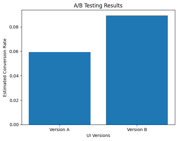
Estimated conversion rate for version A: 0.059
Estimated conversion rate for version B: 0.089

The next step in our A/B test is to conduct a statistical t-test to determine a p-value for whether there is a difference between the two versions. We'll do this using scikit-learn.

from scipy.stats import ttest_ind
successes_a = ab_results[0, ab_results[1, :] == 0]
successes_b = ab_results[0, ab_results[1, :] == 1]

# Perform a two-sample t-test
t_stat, p_value = ttest_ind(successes_a, successes_b)

print(f"T-statistic: {t_stat:.3f}, P-value: {p_value:.3f}")

T-statistic: -18.162, P-value: 0.000

And now, we'll plot our estimated conversion rates.

plt.bar(['Version A', 'Version B'], conversion_rates_estimated)
plt.xlabel("UI Versions")
plt.ylabel("Estimated Conversion Rate")
plt.title("A/B Testing Results")
plt.show()

‍

Thompson Sampling

Now, we'll simulate Thompson Sampling. Check out this post for an explanation of the math behind Coframe's algorithms. In essence, however, we'll again model the “reward” for each variant as a Bernoulli random variable, and keep track of an estimate of the true probability over time.

We apply a beta distribution to model our prior and posterior beliefs for each arm, with two parameters, α, and β. After each trial, Coframe updates this belief based on the result. The beta distribution’s mean is α / (α+β); if the user converts, we increase α, and if they don't, we increase β.

During each step of the Thompson Sampling algorithm, Coframe samples from each distribution and chooses the arm with the highest value to show to the user.

def thompson_sampling(conversion_rates, num_trials):
    successes = np.zeros(num_versions)
    failures = np.zeros(num_versions)
    results = np.zeros((2, num_trials))

    for trial in range(num_trials):
        beta_samples = [np.random.beta(successes[i] + 1, failures[i] + 1) for i in range(num_versions)]
        chosen_version = np.argmax(beta_samples)

        results[1, trial] = chosen_version

        success = np.random.rand() < conversion_rates[chosen_version]
        results[0, trial] = success

        if success:
            successes[chosen_version] += 1
        else:
            failures[chosen_version] += 1

    conversion_rates_estimated = successes / (successes + failures)

    return results, conversion_rates_estimated

ts_results, ts_conversion_rates_estimated = thompson_sampling(conversion_rates, num_trials)

print("Results of each trial (success/failure and chosen version):")
print(ts_results)
print("Estimated conversion rates for each version:", ts_conversion_rates_estimated)

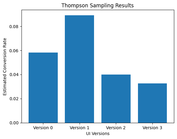
Estimated conversion rates for each version: [0.05815424 0.08914591 0.03982301 0.03252033]

We can also look at how many times each arm was pulled over the 100k trials.

allocations = np.bincount(ts_results[1,:].astype(int))

for i, allocation in enumerate(allocations):
  print (f"Arm {i} was shown {allocation} times.")

Arm 0 was shown 791 times.
Arm 1 was shown 98737 times.
Arm 2 was shown 226 times.
Arm 3 was shown 246 times.

Again, we'll plot the estimated conversion rate for each of the arms.

plt.bar([f'Version {i}' for i in range(num_versions)], ts_conversion_rates_estimated)
plt.xlabel("UI Versions")
plt.ylabel("Estimated Conversion Rate")
plt.title("Thompson Sampling Results")
plt.show()

‍

Comparing the reward over time

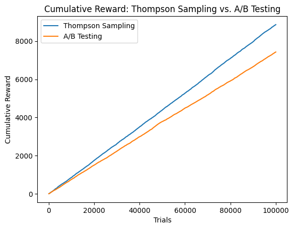
After conducting each of the tests, we'll compare the total reward of each algorithm over time. As a reminder, the "reward" in each trial is 1 if the user was converted, and 0 if the user was not converted. We'll plot the reward of each algorithm over time (they look linear, but they're not up close!)

def cumulative_rewards(results):
    rewards = []
    total_reward = 0
    for result in results:
        total_reward += result
        rewards.append(total_reward)
    return rewards

ab_rewards = cumulative_rewards(ab_results[0,:])
ts_rewards = cumulative_rewards(ts_results[0,:])

colors = ['blue', 'green', 'red', 'orange']


plt.plot(ts_rewards, label="Thompson Sampling")
plt.plot(ab_rewards, label="A/B Testing")
plt.xlabel("Trials")
plt.ylabel("Cumulative Reward")
plt.title("Cumulative Reward: Thompson Sampling vs. A/B Testing")
plt.legend()
plt.show()

‍

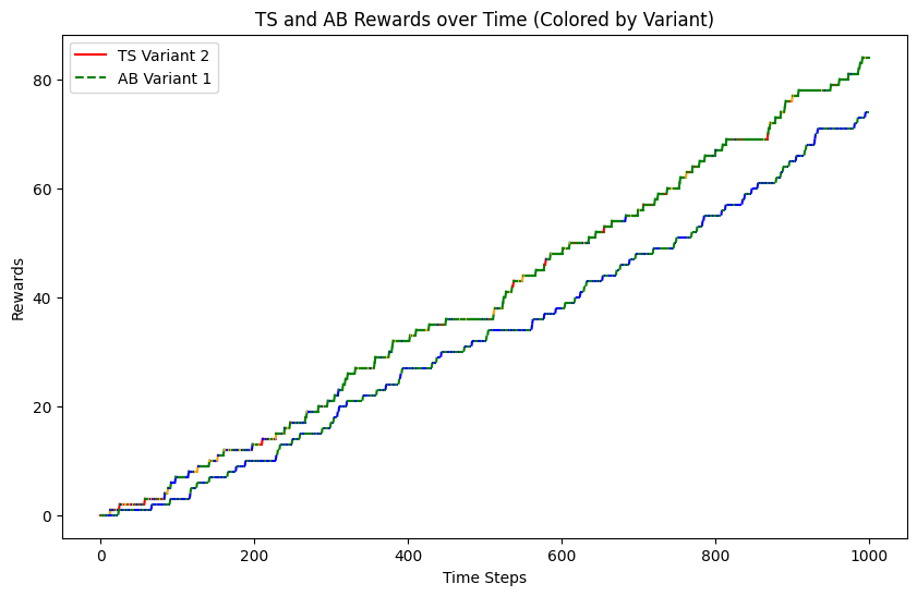
We can also look at the allocations of different arms over time! We'll assign arm 1 the color blue, arm 2 (the best arm) the color green, arm 3 the color red, and arm 4 the color orange. The colors are hard to see with 100k trials, so we'll plot just the first 1000 trials. Notice that while the A/B testing line remains fairly evenly green and blue over time, the TS line slowly turns more and more green as that is discovered to be the best arm.

# Create the figure and axis
fig, ax = plt.subplots(figsize=(10, 6))
colors = ['blue', 'green', 'red', 'orange']

# Plot the Thompson Sampling rewards with color based on variants
for i in range(1000):
    variant = int(ts_results[1, i])
    ax.plot([i, i + 1], [ts_rewards[i], ts_rewards[i + 1]], color=colors[variant], label=f'TS Variant {variant}' if i == 0 else "")

# Plot the A/B rewards with color based on variants
for i in range(1000):
    variant = int(ab_results[1, i])
    ax.plot([i, i + 1], [ab_rewards[i], ab_rewards[i + 1]], color=colors[variant], linestyle='--', label=f'AB Variant {variant}' if i == 0 else "")

# Add labels and title
ax.set_xlabel('Time Steps')
ax.set_ylabel('Rewards')
ax.set_title('TS and AB Rewards over Time (Colored by Variant)')

# Ensure only unique labels are shown
handles, labels = ax.get_legend_handles_labels()
by_label = dict(zip(labels, handles))
ax.legend(by_label.values(), by_label.keys())

# Show the plot
plt.show()

‍

Suppose that each conversion results in, say, $10 of revenue. Then, we can compare the extra revenue brought in by the Thompson sampling algorithm.

extra_revenue = 10 * (ts_rewards[-1] - ab_rewards[-1])
print(f"The Thompson Sampling algorithm brought in ${extra_revenue} in extra revenue, while also comparing 4 variants at once rather than 2.")

The Thompson Sampling algorithm brought in $14350.0 in extra revenue, while also comparing 4 variants at once rather than 2.

Want to play around with the demo yourself? Check out the notebook here.